Dual PRF velocity unfolding

For a radar of wavelength ʎ operating at a fixed sampling period Ʈ_s= 1/PRF, the unambiguous velocity and range intervals are given by the following equation:

V_{u} = \frac{λ}{4 τ_{s}} a n d R_{u} = c \frac{τ_{s}}{2}

where c is the speed of light. Often these intervals do not fully cover the span of velocity and range that one would like to measure. The problem is generally worse for short wavelength radars, since that unambiguous velocity span is directly proportional to ʎ for a given Ʈ_s. If the unambiguous range interval is made sufficiently large by increasing Ʈ_s, then the resulting velocity span may be unacceptably small.

RVP10 provides a built-in mechanism for extending the unambiguous velocity span by a factor of two, three, or four beyond that given above. The technique, called Dual PRF velocity unfolding, uses two pulse periods rather than one, and relies on the extra information thus obtained to correct (that is, unfold) the mean velocity measurement from each individual period. The Dual PRF trigger pattern consists of alternating (N+k)-pulse intervals where the period in each interval is either Ʈ_l (for the low-PRF) or Ʈ_h (for the high-PRF). Here N is the sample size, and k represents a delay that permits the clutter filter to equilibrate to the new PRF after each change. The clutter filter impulse response lengths vary according to which filter is selected.

The two trigger periods Ʈ_l and Ʈ_h must be chosen in either a 3:2, 4:3, or 5:4 ratio. These ratios give factors of two, three, and four times velocity expansion over the Ʈ_h period alone. The unfolding algorithm makes use of the following results. Suppose that the radar observes a target with mean velocity V at each of the two trigger periods. The measured phase angles for the R₁autocorrelations at the two PRFs are:

θ_{l} = \frac{4 π V τ_{l}}{λ} a n d θ_{h} = \frac{4 π V τ_{h}}{λ}

where angles outside the basic [- π, π] interval are returned to that interval by appropriate additions of ± 2π . These angles correspond to the ordinary single-PRF Doppler velocity measurements, and the ± 2π uncertainties reflects the fact that each measurement is folded into its own unambiguous interval:

V_{u l} = \frac{λ}{4 τ_{l}} a n d V_{u h} = \frac{λ}{4 τ_{h}}

If we define φ to be the difference between the two measured phases then:

ϕ = θ_{l} - θ_{h} = \frac{4 π}{λ} [τ_{l} - τ_{h}] V

which can be interpreted as a phase angle within the unfolded interval:

V_{u} u n f o l d = \frac{λ}{4 (τ_{l} - τ_{h})}

Now if Ʈ_l and Ʈ_h are in a 3:2 ratio, then:

τ_{l} - τ_{h} = \frac{τ_{l}}{3} = \frac{τ_{h}}{2}

and thus:

V_{u} u n f o l d = 3 V_{u l} = 2 V_{u h}

The angle Ø represents a velocity phase angle in [- π, π] , but with respect to an enlarged unambiguous interval. By differencing the folded angles from the high and low PRFs, we obtain an angle that is unfolded to a larger velocity span. Similar reasoning shows that the 4:3 ratio gives a factor of three improvement over V_uh, and 5:4 gives a factor of four.

Velocity estimator

In practice, the unfolded angle Ø is not in itself a suitable velocity estimator. This is because the variance of Ø is equal to the sum of the variances of each of its components, that is, twice that of the individual measurements alone. If the target is at all noisy, then this increase in variance can be severe. Rather than use Ø directly, RVP10 uses it only as a rough estimate in determining how to unfold the individual velocity measured from each PRF.

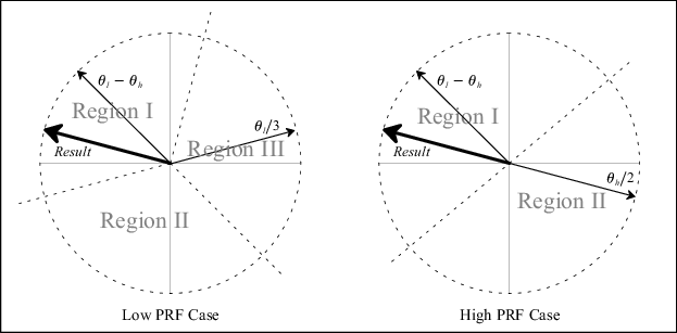
This technique is illustrated in Dual PRF concepts. The figure shows how the low-PRF and high-PRF angles are unfolded based on the difference angle. The diagrams show phase planes representing the large unfolded velocity interval, and the locations of vectors on those planes. In the diagram on the right, the difference angle is plotted, and the plane is divided into two equal size regions, one of which is centered on the difference vector. The high-PRF angle is then divided by two and plotted. The resultant unfolded velocity angle must either be this vector, or this vector plus. Since adding places the vector into acceptance Region 1, where it is nearest the difference angle, it can be concluded that this is the correct unfolding. Likewise, on the diagram on the left, we unfold the low-PRF angle by dividing the plane into thirds centered on the difference angle. The result angle is one of the following equations, depending on which one falls into the acceptance Region 1. The resultant angle is the same in each case.

\frac{θ_{l}}{3}, \frac{θ_{l}}{3} + \frac{2 π}{3} o r \frac{θ_{l}}{3} + \frac{4 π}{3}

RVP10 makes efficient use of the incoming data by unfolding velocities from both the low and the high-PRF data, making use each time of information in the previous ray. When low-PRF data is taken the derived velocities are unfolded by combining information from the previous high-PRF interval. Likewise, when high-PRF data are acquired the velocities are unfolded based on the previous low-PRF interval. Thus, when operating in the Dual PRF mode, RVP10 outputs one data ray for each (N+k)-pulse interval. However, the velocity data in the Dual PRF rays are unfolded, so that the [-1,+1] interval now represents either two or three times the prior velocity range. Put another way, the data are still interpreted as described in the section on mean velocity estimation, except that V_u is now larger.

Width data

The width data is modified during Dual PRF unfolding.

Although valid widths are obtained independently on all rays, those measured at low-PRF are larger than those at high-PRF. This is because the dimensionless width units are with respect to a larger velocity interval in the latter case. To compensate for this, low-PRF widths are multiplied by either 2/3 or 3/4 before being output. This puts them in the same scale as the high-PRF values, and thus, the widths do not vary on alternate pulses. A useful consequence of this is that width data can be sent directly to a color display generator without having to plot every other ray in a different scale.

Limitations of Dual PRF processing

The unfolding algorithms make the assumption that targets are more or less continuous from ray to ray. Otherwise, it would not make sense to use data from a previous ray to unfold velocities in the current ray. You must ensure that their antenna scan rate and beamwidth are such that each target is illuminated, at least partially, over each full 2(N+k)-pulse interval. In practice, a certain amount of decorrelation from ray to ray is acceptable, since the previous rays are used only to decide into which unfolded interval the current ray should be placed. Small errors in the previous ray data, therefore, cause no error in the output. However, large previous-ray errors would lead to incorrect unfolding.

A more subtle side effect of Dual PRF processing arises from clutter filtering because clutter notches now appear at several locations in the unfolded velocity span, rather than just at zero velocity. These additional rejection points come about because the original velocity intervals are mapped some integer number of times to create the unfolded interval.

Since each original interval has a clutter notch at DC, it follows that the final expanded velocity interval has several such notches. For example, in the 3:2 case, in addition to removing DC, the clutter filter removes velocities at - 2V_u/3, + 2V_u/3, and V_u.

These clutter filter "images" are a consequence of the Dual PRF processing technique and are not easily removed. They can cause trouble for the velocity unfolding itself, and they may cause the computed clutter corrections to be wrong at the image points.

To minimize their impact, turn the clutter filter off at far ranges where little clutter is expected, and use a narrow clutter filter.

The 4:3 and 5:4 PRF unfolding ratios are more susceptible to unfolding errors in cases where the spectrum width is large and/or the SNR is low. You must experiment with these ratios to determine which provides the best results for their particular application. Although the RVP10 trigger generator can produce any trigger frequency, only the 3:2, 4:3, and 5:4 ratios can be used with the built-in unfolding algorithms. The RVP10 still permits other PRT ratios to be explored, but the unfolding technique must then be manually programmed on your host computer.

Example

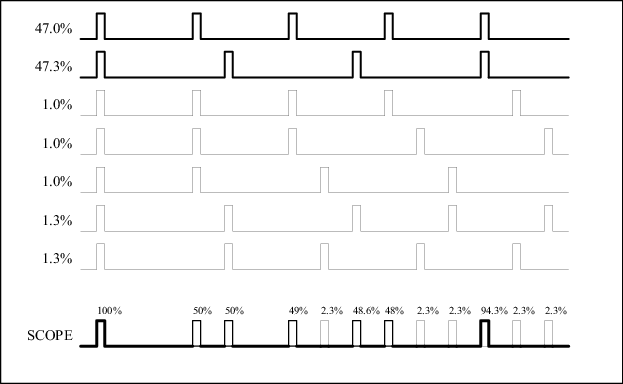
The following example shows seven possible oscilloscope traces (and their associated probabilities) for the RVP10 trigger during Dual PRF operation.

The PRF ratio is 4:3, and the sample size is 50 pulses at the high PRF, and 37 pulses at the low PRF. The signal labeled SCOPE is the composite of these traces, and is what is shown on an oscilloscope.

Note that there are a number of low probability pulses. The exact details of the sample sizes and the trigger hold-off time can make the low probability pulses appear to come and go randomly. This is normal and no cause for alarm.

Figure 2. Example of Dual PRF trigger waveforms