
Plot method for calibration of Io
This approach generates the curve (red) that
determines the value of Io.
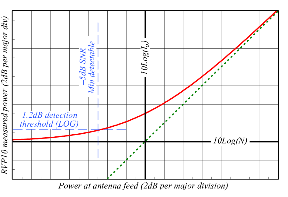
The procedure is to connect a calibrated signal generator to the radar receiver and inject known power levels to generate a calibration plot of measured power versus the inserted power at the antenna feed, similar to that in shown in the figure.
The calibration reflectivity
dBZo is computed from the radar constant and the value of
Io, which is the intercept of the straight line fit (green)
with the noise level.
To understand why this geometric construction
yields the value of Io, let GdB
represent the overall gain of the RF and IF components leading up to RVP10. The green line
can be interpreted as the response of an ideal noise-free amplifier having gain GdB, while
the red curve is the response of the real-world amplifier(s) whose equivalent front-end
noise is Io:
(Red)   10log10(POUT) =  GdB + 10log10( PIN + I0)
(Green) 10log10(POUT) =  GdB + 10log10( PIN )
The measured receiver noise is the horizontal asymptote of the red curve, that is, the value
of the red curve when the input power PIN is 0:
10log10(N) = GdB + 10log10(I0)Intersecting this measured noise level with the green straight line gives:
GdB + 10log10(I0) = GdB + 10log10(PIN )From which we see that the input power at the point of intersection is, indeed,
Io.
Io is the
received signal level that produces 0 dB SNR, that is, signal power equal to noise power. Do
not confuse this with the minimum detectable power PMDS which
typically is several dB lower, depending on processor settings. In the above example, a 1.2
dB LOG detection threshold is shown (horizontal blue line) for the
received signal. If RVP10 applies sufficient range and time averaging so that thermal noise
alone produces very few false alarms above 1.2 dB, then PMDS are
a 5dB lower than Io. We would expect a detection rate of roughly
50% for echoes arriving at this "minimum detectable" level.
Typically a CW test signal is used to generate the test curve shown in the figure. Follow the instructions provided by the radar manufacturer for injecting a test signal. During calibration, the radar should be fully operational, so that all sources of noise are present. Ideally the transmitter should be turned on during calibration.
 | Caution Verify with the radar manufacturer that no damage can occur to the signal generator if the transmitter is running during the calibration. |
- Raise the antenna up a few degrees to avoid ground thermal noise.
- Insert signals at steps of 5 or 10 dB over the entire range of the system.
-
Draw the plot shown in the previous figure.
You can use fine resolution steps at the ends of the scale to observer the details of the roll off.

If you are using the IRIS software, you can do this in the Zauto utility. -
Tune the frequency of the signal generator using the setup command pr, and displaying the received signal spectrum.
Check the tuning at the end of the calibration to make sure the signal generator and IFDR have not drifted apart.
Each time that a new signal level is injected, the measured power values are obtained by first invoking the SNOISE command and then reading- back the results using the GPARM command. Use the
Log of Measured Noise
              Level (Word 6)
from GPARM.This procedure averages many samples together.
-
Turn it all the way down and make one more sample to measure the noise level
N.
You can obtain
Iofrom the intercept of the horizontal line at N and the straight line fit to the linear portion of the curve. - Correct the value for losses.