
Frequency Domain Processing- Doppler power spectrum
The Doppler power spectrum (also known as Doppler spectrum) is the easiest way to visualize the meteorological information content of the time series.
The Doppler power spectrum is obtained by taking the magnitude squared of the input time series, that is, for a continuous time series,
Here S denotes the power
spectrum as a function of frequency ω, and f denotes the Fourier transform of
the continuous complex time series s(t). The Doppler power spectrum is
real-valued since it is the magnitude squared of the complex Fourier transform of
s(t).
In practice, a pulsed radar operates with discrete rather than continuous time series. That is, there is an I and Q value for each range bin for each pulse. In this case we use the discrete Fourier transform or DFT to calculate the discrete power spectrum.
When we have 2n input time
series samples (for example, 16, 32, 64, 128, ...), we use the fast Fourier transform
algorithm (FFT), which is significantly faster than the full DFT.
The DFT has the form:
Typically a weighting function or "window" wm
is applied to the input time series sm to mitigate the effect of
the DFT assumption of periodic time series. RVP10 supports different windows such as the
Hamming, Blackman, Von Han, exact Blackman, and the rectangular window for which all spectral
components are weighted equally.
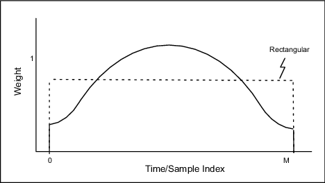
Although the window gain can be adjusted to conserve the total power, there is an effective reduction in the number of samples which increases the variance (or uncertainty) of the moment estimates. For example, the variance of the total power is greater when computed from a spectrum with Blackman weighting compared to using a rectangular window. This is because there are effectively fewer samples due to the de-emphasis of the end points. This is a negative side to using a window.
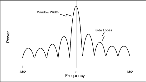
The DFT of the window itself is known as its impulse response which shows all of the frequencies that are generated by the window itself. A generic example is shown in the following figure which illustrates that these side lobe frequencies can have substantial power. This is not a problem for weather signals alone, but if there is strong clutter mixed in, then the side lobe power from the clutter can obscure the weaker weather signals. The rectangular window has the worst sidelobes, but the narrowest window width. However, the rectangular window provides the lowest variance estimates of the moment parameters (in the absence of clutter).
More aggressive windows have lower side lobe power at the expense of a broader impulse response and an increased variance of the moment estimates.
In summary of the DFT approach and spectrum windows:
- When the clutter is strong, an aggressive spectrum window is required to contain the
clutter power so that the side lobes of the window do not mask the weather targets. The side
lobe levels of some common windows are:
- Rectangular 12 dB
- Hamming 40 dB
- Blackman 55 dB
- More aggressive windows typically have a wider impulse response. This effectively increases the spectrum width. Rectangular is narrow, Hamming intermediate, and Blackman the widest.
- Windows effectively reduce the number of samples resulting in higher variance moment estimates. Rectangular is the best case, Hamming is intermediate, and Blackman provides the highest variance moment estimates.
The best approach is to use the least aggressive window possible in order to contain the clutter power that is present. That is, an adaptive approach is the best.