Doppler Spectrum Plot (Spec)

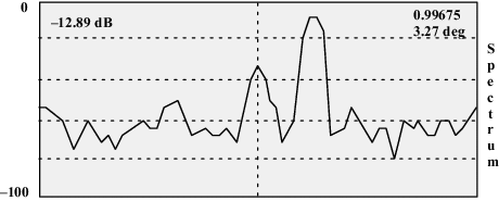
This plot is generated when you choose the Spec plot parameter. This is the most useful plot for monitoring the alignment and performance of the Doppler channel.

The Doppler spectrum is computed from the I and Q time series for the selected range. See Time Series at a Selected Range (I, Q, and LOG).

The FFT mode spectrum can be displayed directly. The scale is in dB marked with 20 dB divisions. Zero velocity is indicated by a vertical line. This is the velocity of ground clutter targets. The Doppler spectrum plot is always given twice as much vertical height on the screen as the other plots.

The numerical values in the display are as follows:

• Top left

  Linear channel power in dB. This is uncalibrated on an absolute scale. However it is very accurate on a relative scale as long as the linear receiver is not saturated.

• Top right

  Signal quality index or SQI (|R1|/R0). This is a value between 0 (white noise) and 1 (pure tone). This is useful in determining the coherency of the radar system. See Ascope checkup procedures.

• Top right (beneath SQI)

  RMS phase noise in degrees. This includes noise contributions caused by both amplitude and phase errors, and is computed directly from the SQI as follows:

  $P h a s e N o i s e = 180 π × − 1 n ( S Q I )$
• Time series are clutter-filtered. You can use the filter fields to see the effect of various filters on the Doppler spectrum.

The typical Doppler spectrum contains white noise at all velocities, a ground clutter spike at 0 velocity, and a weather spectrum. Some points to note:

• With the clutter filter set to None (no filter), you can observe a strong clutter target to determine the linear dynamic range of the system. Observe the dB difference between the peak of the clutter and the white noise.

• Coherent artifacts are caused by leakage of other signals, such as 50 or 60 cycle line power into the transmitter/receiver system. These appear as peaks located symmetrically about 0 velocity.

  To obtain the best Doppler measurements, minimize coherent artifacts by reducing the leakage of stray signals.

• Image spectra occur when a weather spectrum has a mirror image on the other side of zero velocity. Usually the image is smaller than the primary weather peak. Image spectra are typically caused by the following:
  • Saturation of the A/D converters
  • Gain imbalance of the I and Q channels

  To correct these problems, see:

  • Coarse adjustment of gain and offset pots
  • RVP10 User Guide (M212604EN)

The number of points that are plotted are 4, 8, 16, 32, 64, 128, or 256 as indicated by the Spectrum Size field.

You can change the number of points in the Pulse Samples field. If a number other than a power of 2 is entered, the next lowest allowable value is accepted (for example, a Pulse Sample of 126 sets the Spectrum Size field to 64 points).

When selecting the range for the spectrum, it is useful to display a velocity against range (V) or reflectivity against range (Z) plot. These plots can show you where there are targets of interest.

Because spectra can be very noisy, Ascope has a spectrum averaging feature for detecting weak signals. Averaging causes the update rate to slow down. A value of None corresponds to no averaging. 8 is the maximum value.

See also the Pulse Samples, Spectrum Average, Spectrum Window, Doppler and LOG Filter, and Range Strobe fields.