FIR (matched) filter
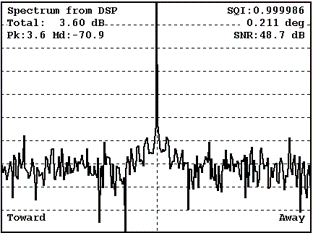
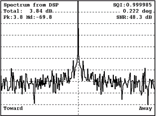
RVP10 includes two methodologies to design a digitally matched filter: the continuous wave (CW) bandpass filter, and the idealized matched filter.
The continuous wave (CW) bandpass filter is the legacy methodology used within RVP900 and older RVP versions. In this method, user defines the filter length (number of taps), center frequency, and bandwidth.
The idealized matched filter is a new method. It is calculated by taking the conjugated
transmit waveform and applying a windowing to the pn
samples.
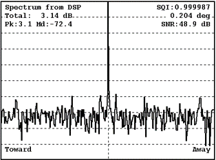
 | For information on designing the digital matched filter using the graphical user interface, see Burst spectra and AFC plot (Ps). |
The legacy bandpass design procedure computes two sets of filter coefficients, and , such that the instantaneous quadrature samples at a given bin are:
,
where N is the length of the
filter. The input samples pn are centered on the range
bin to which the (I, Q) pair is assigned. Note
that some pn may overlap among adjacent bins. That is,
the filter length may be greater than the bin spacing. The overlap introduces a
slight correlation between successive bins, but the longer length allows a better
filter to be designed. In the situation where the filter length design is smaller
than the bin spacing, remaining samples pn are skipped
until the start of the next range bin. In the legacy bandpass filter, Vaisala
generally recommends the filter length be about 1.5 x the pulse length.
The sums above for I and Q are computed on RVP10 using a flexible FGPA that can perform billions of sums of products per second.
Reference phase
The reference phase for each transmitted pulse
is computed using the same two FIR sums, except that bn
is substituted for pn and choices of window function are
either Rectangular, Hamming, or Blackman.
For magnetron systems, the N
bn samples are centered on the transmitted burst.
For Klystron systems, the N bn
samples may be obtained from the burst pulse (recommended) or
from the CW STALO. If the Klystron is phase modulated by an external phase shifter
(instead of the IFDR digital transmitter board), the samples must be from the
modulated STALO.
Coefficients
The coefficients are computed as:
where fIF
is the radar intermediate frequency,
fSAMP is the IFDR sampling
frequency, and ln represents the
coefficients of an N-point symmetric low-pass FIR filter that is matched to the
bandwidth of the transmitted pulse. The multiplication of the
ln terms by the
sin() terms effectively converts the low-pass filter to a
band-pass filter centered at the radar IF.
The formula for the coefficients is identical except that
sin() is replaced with cos().
The phase of the sinusoid terms, and
the symmetry of the ln terms, has been chosen to have a
valuable overall symmetry property when n is replaced with
(N-1)-n, that is, the sequence is reversed:
The coefficients needed to compute I are the reverse of the
i coefficients needed to compute Q. That is,
if you know fi n, then you also know
fqn.
When selecting to use the idealized matching filter, the
ficoefficients are computed similarly, except that the symmetric
low-pass FIR filter ln is replaced by a scaling function
so the gain/loss at the center frequency is 0 dB, and W[n] and windowing
function.
Windowing functions
W[n] are a signal shaping technique by increasingly reducing
the amplitudes of samples from the center to the edge of the time domain. They may
be used to increase signal coherency, which improves ground clutter suppression, or
to increase the differentiation of 1st trip from multi-trip echo or from other types
of interference. However, applying a windowing function will also generally decrease
sensitivity and increase the variability seen in the final data types from the
signal processor. For more information on windowing functions, see Frequency Domain Processing- Doppler power spectrum.
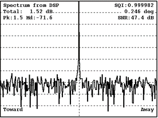
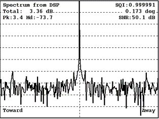
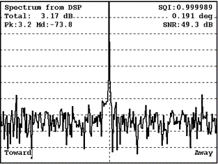
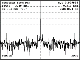
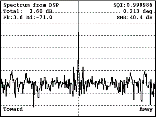
The types of windowing functions supported within the matched filter are Rectangular (no window), Triangular, Hann, Hamming, Blackman, Blackman Exact, Tukey, Kaiser, and Flat top. For any given noise bandwidth, the Rectangular window function provides the lowest root mean square error of the data estimates, and the Triangular window provides the best signal coherency.
|
|
||||||||||||||||||||||||||||||||||||||||||||
|
|
||||||||||||||||||||||||||||||||||||||||||||
|
|
||||||||||||||||||||||||||||||||||||||||||||
|
|
||||||||||||||||||||||||||||||||||||||||||||