NDOP Display and Algorithm

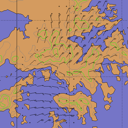
The following example is an actual NDOP display showing the low-level (1 km) winds for a projection 40 km (24.9 mi) across using two S-band radar systems. ¹

The meteorological situation is an event of strong Northerly winter monsoon flow over China colliding with Easterlies over the sea. The overlay map shows the contours of the mountainous terrain North of Hong Kong. Note the 50 knot winds funnelling through the mountain pass to the North of Hong Kong.

The "+" points in the display show the regions where the crossing angle criterion was met. These regions are on either side of the baseline that connects the 2 radars. However, if there are no weather targets, a wind cannot be calculated.

The algorithm takes the following steps to compute the grid point winds:

1. Create 3D CAPPI products of radial velocity for the 2 radars in the common projection at the grid height spacing.

   The horizontal resolution of the CAPPI products is subject to the following constraints:

   • The resolution of the CAPPI pixels is set to be twice the spacing of the input radial velocity data. For example, for 125-m (410 ft i in) input bins, the CAPPI resolution is set to 250 m (820 ft 3 in).

   • The number of CAPPI pixels for each output resolution grid element should be at least 9 (3 × 3).

     If this is not the case, then the resolution of the CAPPI is increased.

     In the same example, if the output resolution were 2 km (1.2 mi) then per the 250-m (820 ft 3 in) pixel spacing in (1) there would be 8 × 8 = 32 pixels for each output grid point.

   • The maximum number of pixels in the CAPPI is 1100 × 1100. The CAPPI is clipped at this value.

     For a 40 km (24.9 mi) range span (80 km (49.7 mi) total across the output array), there would be (4 pixels/km)*80 (km) = 320 pixels in the CAPPI (320 × 320 for a square projection).

2. The data from the radial velocity CAPPI products are processed with the multiple Doppler algorithms to obtain a grid of (x,y) wind vectors at the original CAPPI resolution (for example, 320 × 320).

3. The high-density wind vectors are averaged to reduce the data to the final output grid.

   Continuing the example, with 4 pixels per km in the CAPPI and a an output resolution of 2 km (1.2 mi), we would average 8 × 8 = 32 wind vectors for each output grid point.

4. To eliminate noise and speckle effects, a grid point is thresholded if there are fewer than 3 values to average or less than 25 % coverage.

   In the example, the 25 % would correspond to 8 wind estimates.

When the vector averages are computed, a Wind Quality Index (WQI) is also calculated and stored with the data. This is used for thresholding when the product is displayed.

The WQI is computed from the variances #sigma#2x and¨#sigma#2y of the individual components of each (x,y) wind vector that is computed from the CAPPI data. For every CAPPI velocity pair that contributes to the final X and Y wind, the 2 variance terms are also computed so that WQI can be derived as:

where $V n o r m$V_norm is a normalization term, and is the standard deviation that would result if uniformly distributed random vectors at half the Nyquist velocity were input to the algorithm, that is, that case would produce a WQI of 0.

where $V 1 u$ and $V 2 u$ are the Nyquist velocities for the two CAPPI input products.