

SHEAR Algorithm
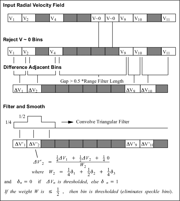
The SHEAR algorithm shown in the following figure is for radial shear. The azimuth shear is similar in "B-scan" space (range-azimuth).
Point Clutter Bin Removal
Point clutter bins produce erroneous high shear values when they are differenced with surrounding valid velocities. The first step in the shear algorithm is to remove obvious clutter bins which were not canceled by the signal processor clutter filter. All velocity bins having a velocity within 2 % of 0 velocity (as compared to the full velocity range) are tagged as potential Clutter Bins. A Clutter Length Scale is defined as 1/3 of the Range Filter Length value in km. Contiguous runs of Clutter Bins that are less than or equal to the Clutter Length Scale are rejected.
For example, suppose the bin spacing and Range Filter Length values are selected so that Clutter Length Scale corresponds to 3 range bins. Then any single isolated Clutter Bin would be rejected, as would runs of 2 or 3 clutter bins. Runs of 4 or more clutter bins would not be rejected because they are interpreted as real weather.
Regardless of the Clutter Length Scale, isolated clutter bins (single bins) are always removed.
Differencing (radial difference example)
The next step is to perform the range differencing of the radial velocities. The radial wind shear algorithm computes the shear by taking the bin-to-bin difference on a PPI surface.
If the differencing algorithm encounters a blank bin, it skips out in range to the next valid bin to take a difference, provided the bin is within 0.5*Range Filter Length.
For example, if the Range Filter is set to correspond to 3 bins, the differencing algorithm differences over a gap of one bin, but not over a gap of 2 or more bins. The velocity differences are placed as close as possible to the center of the difference interval, to the nearest bin that is less than or equal to half of the difference interval.
Smooth the Differences
Differencing is inherently noisy. The next step is to smooth the computed differences. This not only reduces the noise, it also fills in small gaps of missing bins and cancels any remaining isolated bins.
The smoothing algorithm uses a triangular window whose total width is equal to the Range Filter Length value. The sum of the weights defined by the triangular filter is always 1 unless a bin is thresholded.
In the previous figure, the Range Filter Length corresponds to 3 bins. Each velocity in the filter range is multiplied by the corresponding weight and then summed. The mean is obtained by dividing by the total weight. Thresholded bins are not weighted. If the total weight is less than or equal to 0.5, the shear value is rejected. This eliminates isolated bins. This approach can also fill gaps. A longer range filter rejects a longer run of isolated bins and fills a longer gap.
Azimuth Shear Calculation
The following figure is a depiction of "B-Scan" space (a PPI surface). The coordinates are range and azimuth. The radial shear is obtained by differencing in range along a radial.
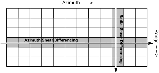
The azimuth shear algorithm is analogous to the radial shear algorithm except that:
- Differencing is performed from ray-to-ray at constant range.
- The azimuth filter length is specified in degrees.
- The final azimuth values are range normalized and corrected for the apparent azimuth shear caused by the mean wind. The mean wind value is obtained from the VVP algorithm. This correction is an optional step.
For information on the mean velocity correction, see Optimizing SHEAR for Microburst Detection.
Shear Magnitude
After both the radial and azimuth shears have been obtained, the next step is to compute the shear magnitude. This is the square root of the sum of the squares of the 2 shear values (radial and azimuth) associated with each bin.
If only a single shear is selected (radial or azimuth), this step is skipped.
Convert to Cartesian and Optional Final Cartesian Smoothing
The conversion to Cartesian transforms the B-scan values of the shear magnitude to X-Y coordinates.
The algorithm is identical to the PPI algorithm, which uses a last-in approach for both range and azimuth filling. An optional 2D smoother with selectable length scale can be passed over the data at this point.